

Method

Point-Aware Self-Supervised Visual Odometry with Rotation-Decoupled Pose Learning [PAVO]
Code will be released upon publication.

Submitted on 14 Jul. 2026 07:58 by
Hongyuan Zhao (Beijing Institute of Technology)

Running time:0.02 s
Environment:GPU @ 2.5 Ghz (Python)

Method Description:
PAVO is a lightweight self-supervised monocular
visual odometry method that predicts relative
camera motion from consecutive left color images.
The method builds on a SC-Depth-style depth-pose
framework and introduces point-aware pose learning
through learned matching confidence, motion-
descriptor residual guidance, and a rotation-
decoupled ARN branch. During inference, PAVO
performs single-pass pose prediction without
stereo input, LiDAR, loop closure, bundle
adjustment, or factor graph optimization. The
submitted trajectories are generated by
sequentially composing the predicted frame-to-
frame poses with the same model parameters for all
KITTI test sequences.
Parameters:
Input: monocular left color images only.
Training data: KITTI odometry sequences 00–08.
Test data: KITTI odometry sequences 11–21.
Image resolution: 640 x 192.
Backbone: ConvNeXtV2-Atto with 1/8-resolution pose
feature stage.
Pose estimation: direct frame-to-frame regression,
no test-time BA, no factor graph, no loop closure.
Matching guidance: confidence residual + gated
motion-descriptor residual.
ARN branch: rotation-decoupled auxiliary rotation
head.
Depth range: 0.1–100 m.
Same parameters are used for all submitted
sequences.
Latex Bibtex:
@misc{anonymous2026pavo,
title = {Point-Aware Self-Supervised
Visual Odometry with Rotation-Decoupled Pose
Learning},
author = {Anonymous},
year = {2026},
note = {Manuscript under double-blind
review}
}

Detailed Results

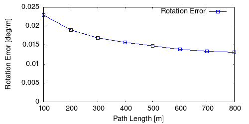
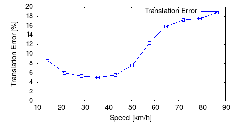
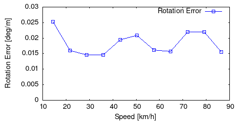
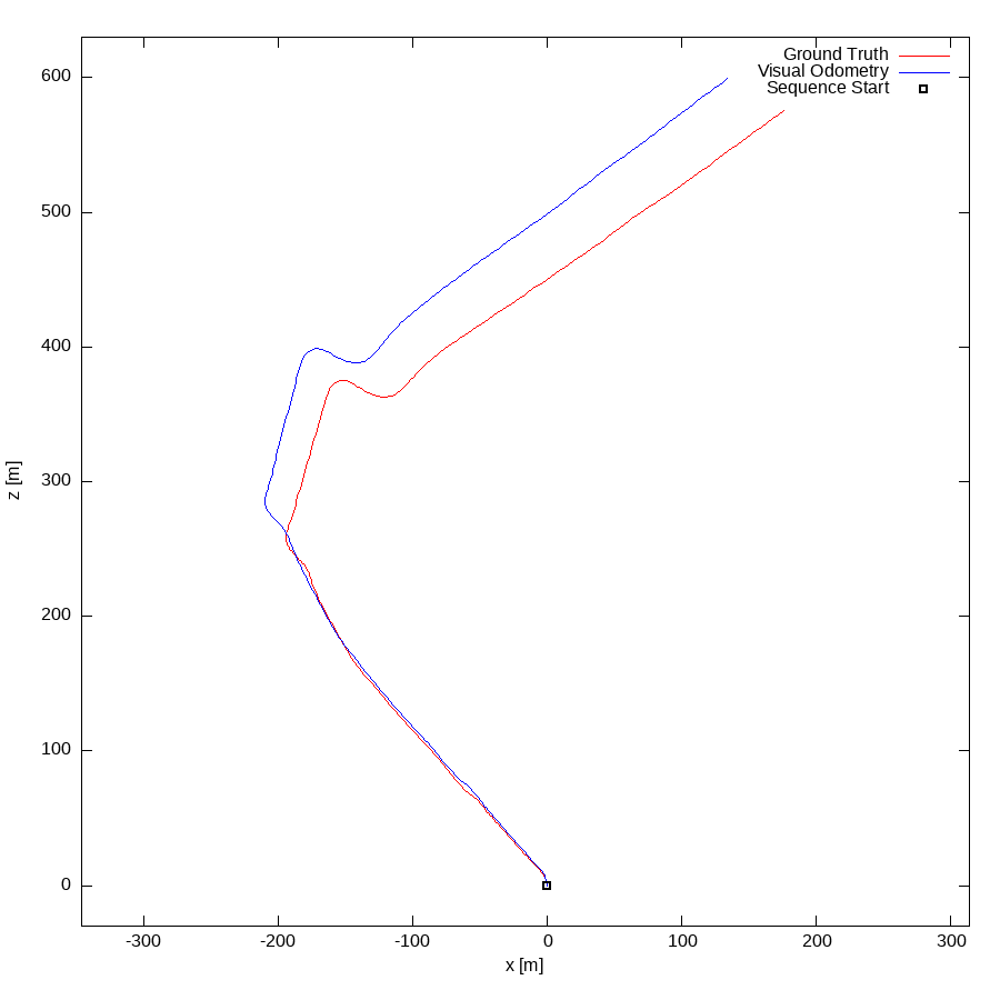
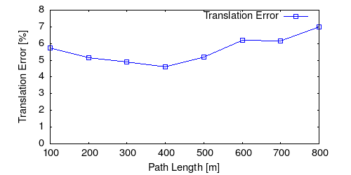
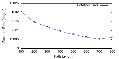
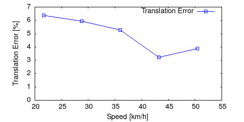
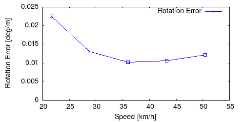
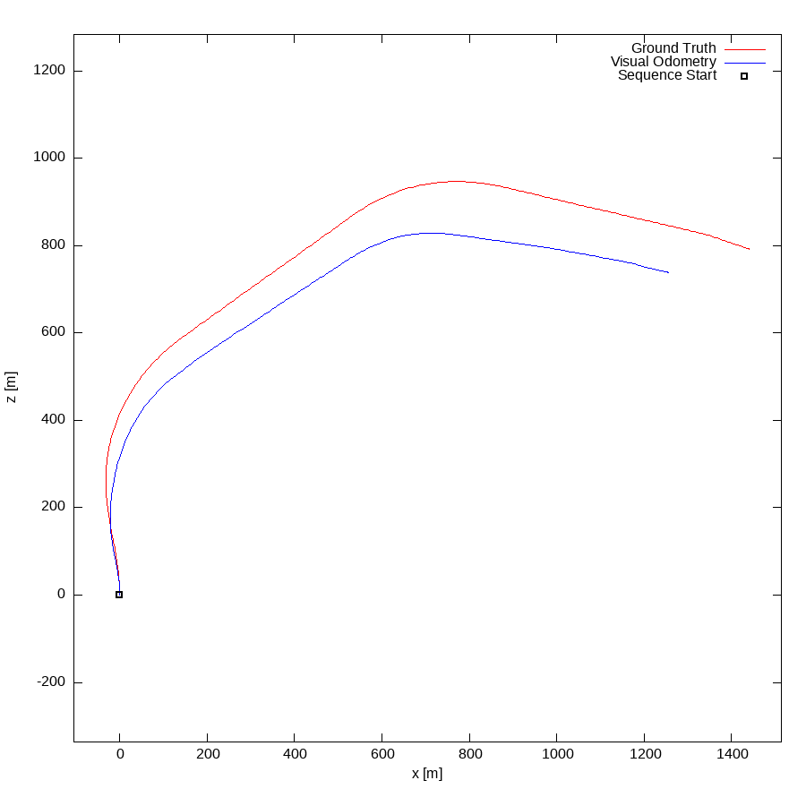
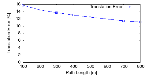
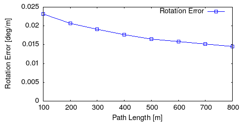
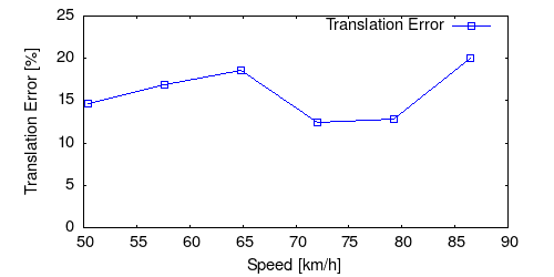
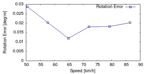
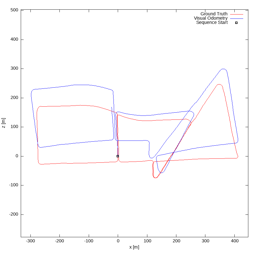
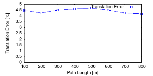
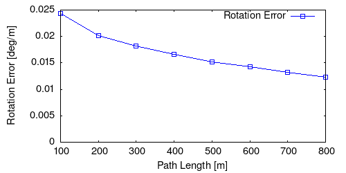
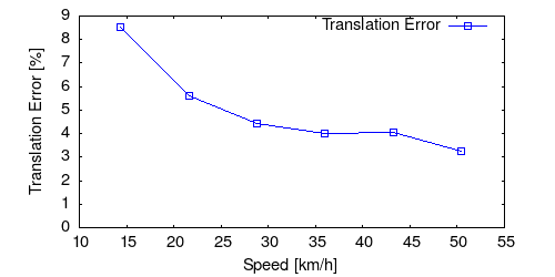
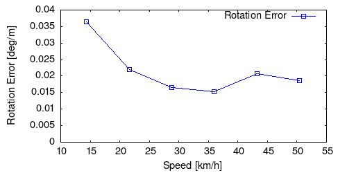
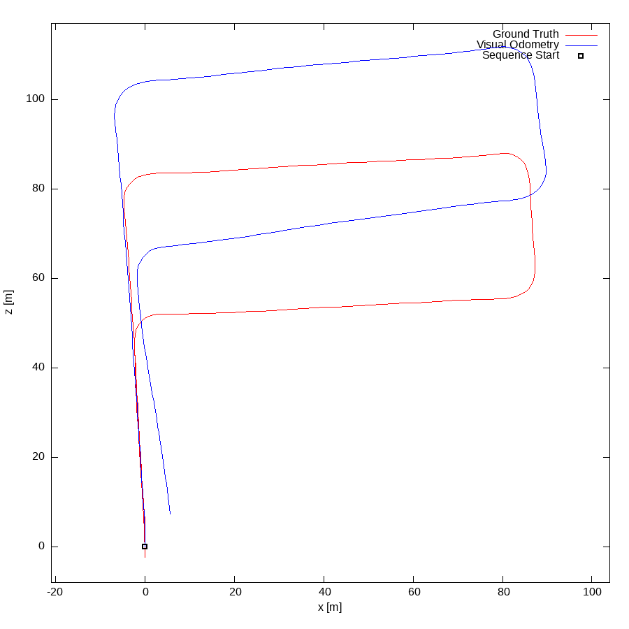
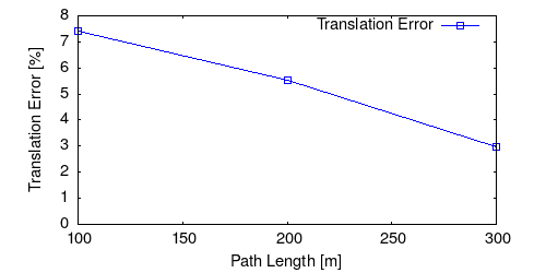
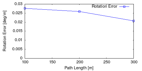
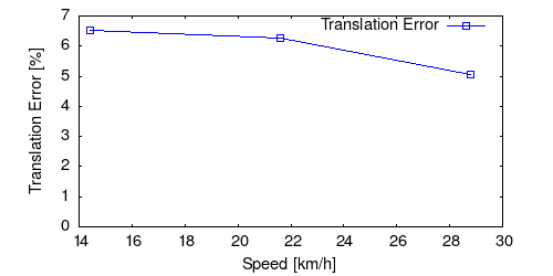
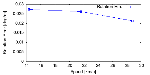
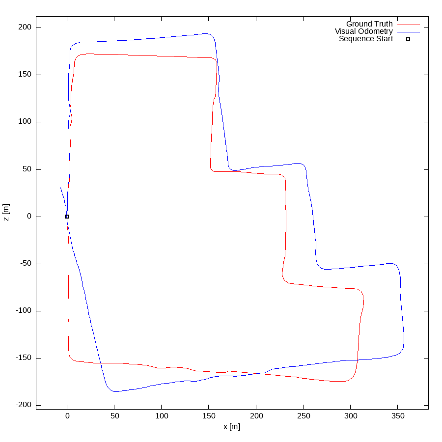
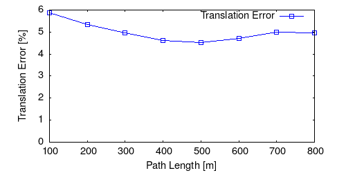
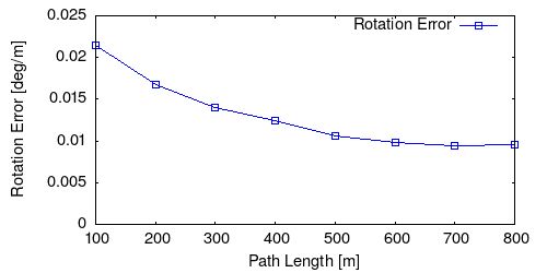
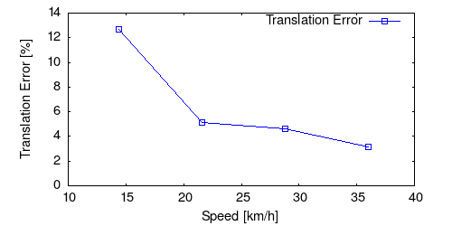
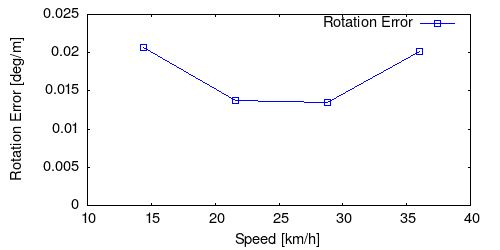
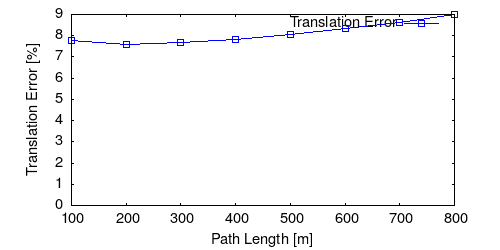
From all test sequences (sequences 11-21), our benchmark computes translational and rotational errors for all possible subsequences of length (5,10,50,100,150,...,400) meters. Our evaluation ranks methods according to the average of those values, where errors are measured in percent (for translation) and in degrees per meter (for rotation). Details for different trajectory lengths and driving speeds can be found in the plots underneath. Furthermore, the first 5 test trajectories and error plots are shown below.

Test Set Average

This figure as: png eps txt gnuplot


This figure as: png eps txt gnuplot


This figure as: png eps txt gnuplot


This figure as: png eps txt gnuplot


Sequence 11


This figure as: png eps txt gnuplot


This figure as: png eps txt gnuplot


This figure as: png eps txt gnuplot


This figure as: png eps txt gnuplot


This figure as: png eps txt gnuplot


Sequence 12


This figure as: png eps txt gnuplot


This figure as: png eps txt gnuplot


This figure as: png eps txt gnuplot


This figure as: png eps txt gnuplot


This figure as: png eps txt gnuplot


Sequence 13


This figure as: png eps txt gnuplot


This figure as: png eps txt gnuplot


This figure as: png eps txt gnuplot


This figure as: png eps txt gnuplot


This figure as: png eps txt gnuplot


Sequence 14


This figure as: png eps txt gnuplot


This figure as: png eps txt gnuplot


This figure as: png eps txt gnuplot


This figure as: png eps txt gnuplot


This figure as: png eps txt gnuplot


Sequence 15


This figure as: png eps txt gnuplot


This figure as: png eps txt gnuplot


This figure as: png eps txt gnuplot


This figure as: png eps txt gnuplot


This figure as: png eps txt gnuplot


eXTReMe Tracker