The KITTI Vision Benchmark Suite

Method

Lidar-Monocular Visual Odometry [la] [LIMO]
https://github.com/johannes-graeter/limo

Submitted on 24 Feb. 2018 10:30 by
Johannes Gräter (Institute of Measurement and Control, Karlsruhe Initute of Technology)

Running time:		0.2 s
Environment:		2 cores @ 2.5 Ghz (C/C++)

Method Description:

This is a follow up of Liviodo. We use Lidar to extract depth for feature point tracks from a monocular cmaera. Drift is reduced using keyframe-based bundle adjustment.

Parameters:

depth_loss=0.16
reprojection_loss=1.6
outlier_rejection_quantile=0.95
num_rejection_iterations=2
prior=liviodo

Latex Bibtex:

@ARTICLE{2018arXiv180707524G,
author = {{Graeter}, J. and {Wilczynski}, A. and {Lauer}, M.},
title = "{LIMO: Lidar-Monocular Visual Odometry}",
journal = {ArXiv e-prints},
archivePrefix = "arXiv",
eprint = {1807.07524},
primaryClass = "cs.RO",
keywords = {Computer Science - Robotics, Electrical Engineering and Systems Science - Image and Video Processing},
year = 2018,
month = jul,
adsurl = {http://adsabs.harvard.edu/abs/2018arXiv180707524G},
adsnote = {Provided by the SAO/NASA Astrophysics Data System}
}

Detailed Results

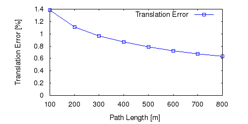
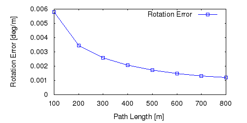
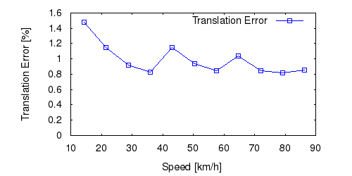
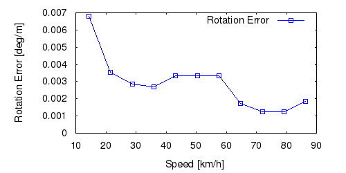
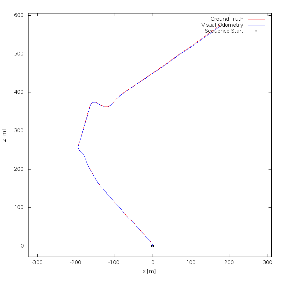
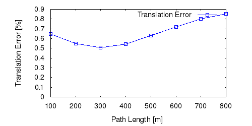
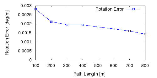
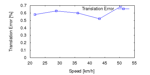
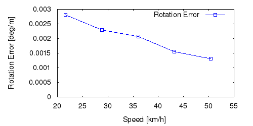
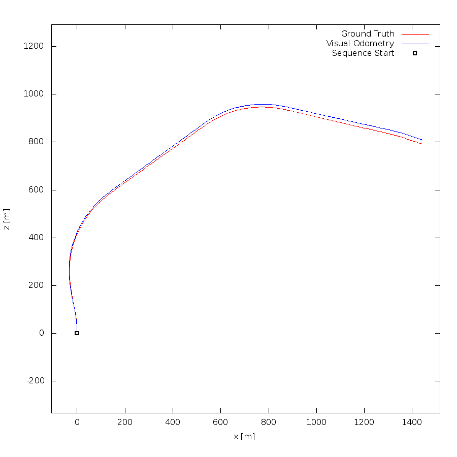
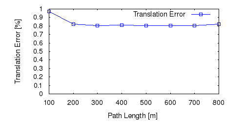
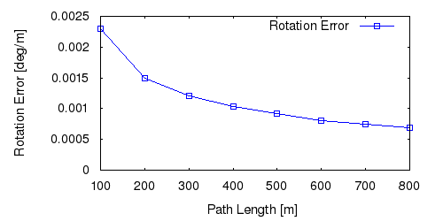
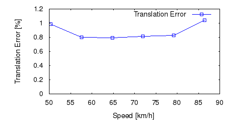
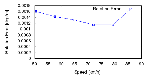
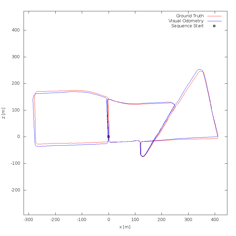
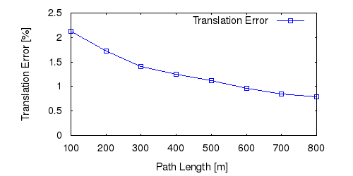
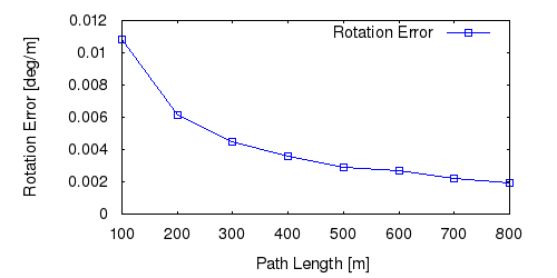
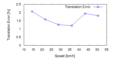
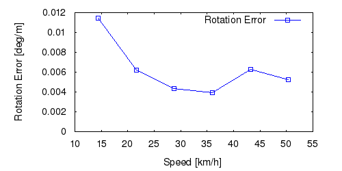
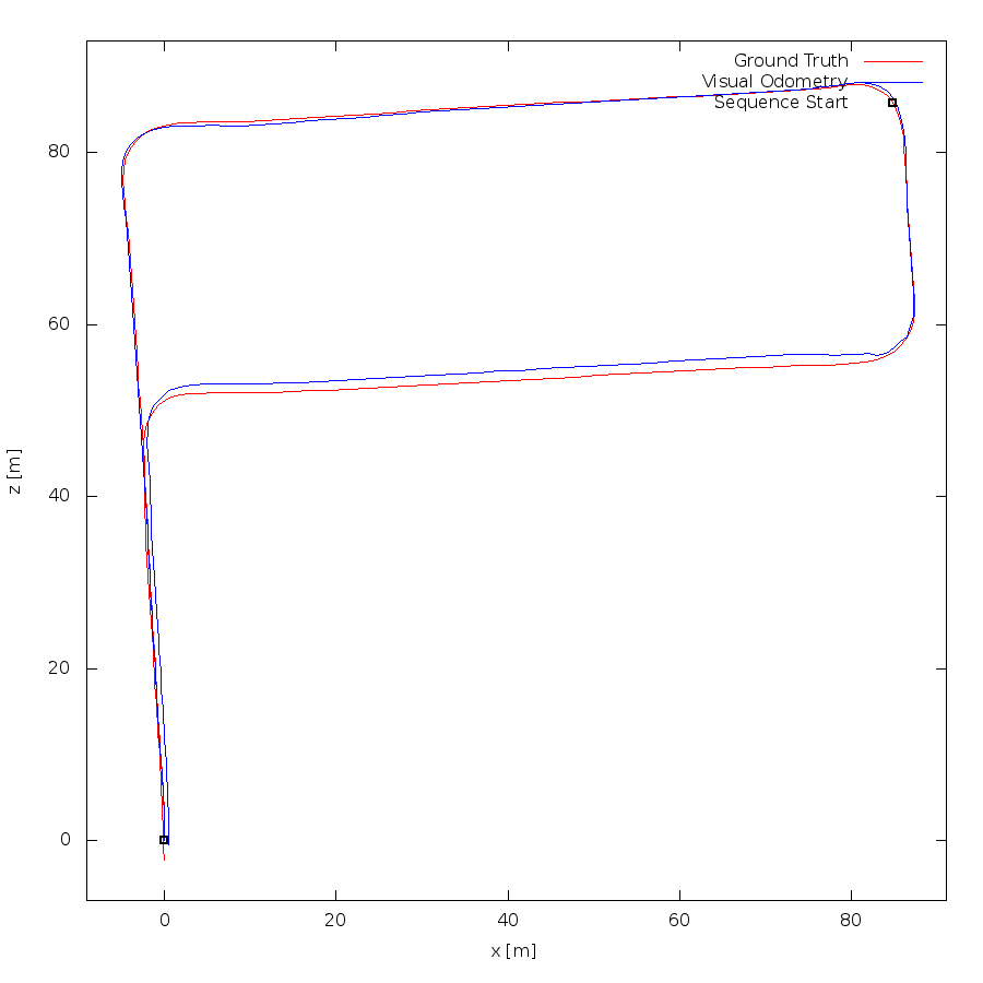
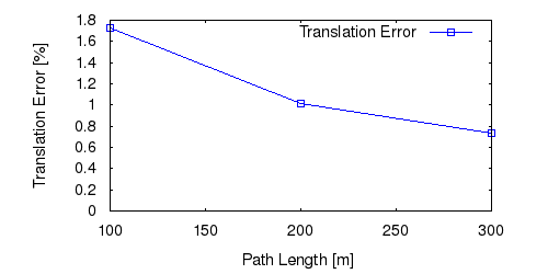
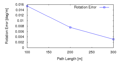
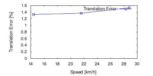
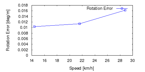
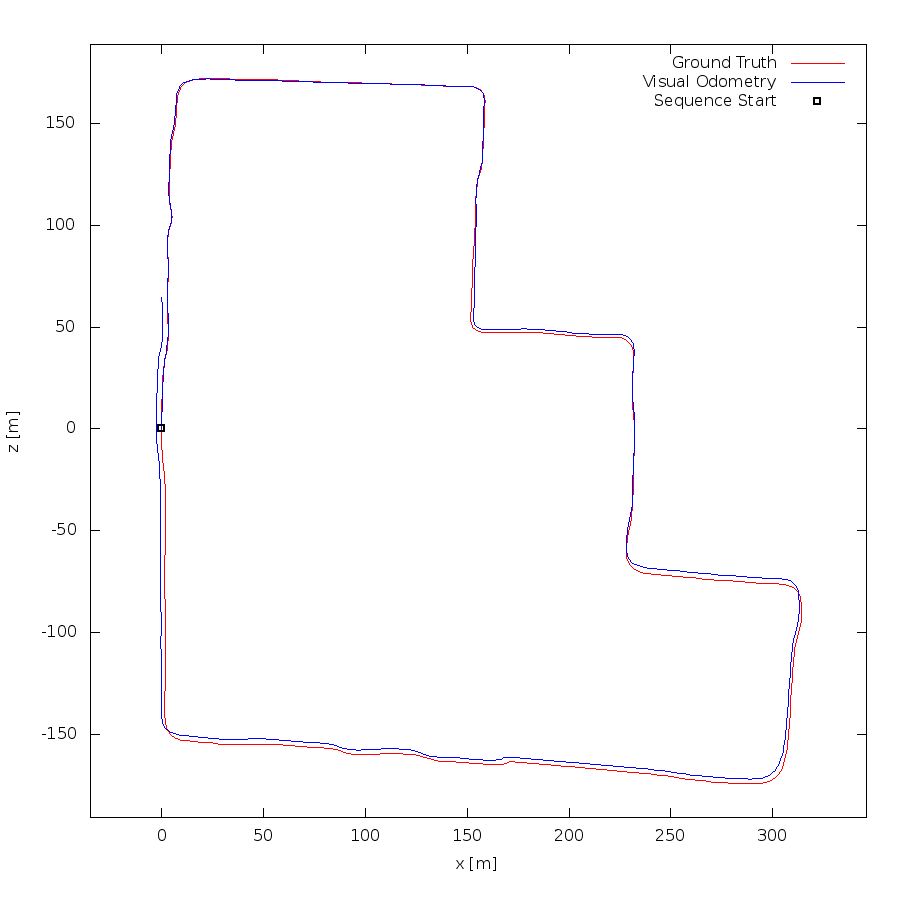
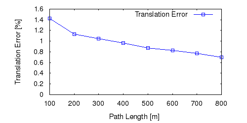
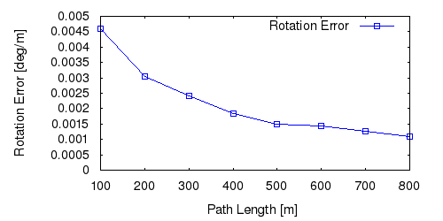
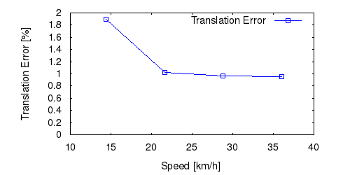
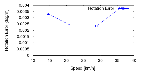
From all test sequences (sequences 11-21), our benchmark computes translational and rotational errors for all possible subsequences of length (5,10,50,100,150,...,400) meters. Our evaluation ranks methods according to the average of those values, where errors are measured in percent (for translation) and in degrees per meter (for rotation). Details for different trajectory lengths and driving speeds can be found in the plots underneath. Furthermore, the first 5 test trajectories and error plots are shown below.